
(BigData Analysis 도전기) Kaggle Geospatial Analysis Tutorial (1. Your First Map)
by 줌코딩
Geospatial Analysis
- 드디어 Pandas 강의를 마치고 본격적으로 Geospatial Analysis 강의이다.
- Geospatial data란 데이터에 지리적인 위치 정보가 있는 것이다.
- 이런 정보들을 분석해서 시각화 하는 방법에 대해서 알아보자.
Introduction
- 이번 course를 통해서 지리 데이터를 처리하고 시각화하는 방법에 대해서 배워볼 것이다.
- 이와 함께, 실생활에서 접할 수 있는 다음과 같은 문제들에 대한 solution을 또한 제공 받을 것이다.
- “세계 비영리 단체가 필리핀 외진 지역의 범위를 확대해야하는 곳은 어디입니까?”
- “위협받는 조류 종인 자주색 마틴은 어떻게 북미와 남미를 여행합니까? 새들이 보존 지역으로 여행합니까?”
- “추가 지진으로 일본의 어느 지역이 혜택을 볼 수 있습니까?”
- “캘리포니아의 어떤 Starbucks 매장이 다음 Starbucks Reserve Roastery 위치의 강력한 후보입니까?”
- “뉴욕시에는 차량 충돌에 대응하기에 충분한 병원이 있습니까? 도시의 어느 지역에 커버리지가 부족합니까?”
- 이번 tutorial에서는 이 course를 따라가기 위한 기본이 되는 geospatial dataset의 시각화를 배워보도록 하자.
Reading data
- geospatial data를 읽어들이기 위해서 GeoPandas library를 활용하도록 하겠다.
import geopandas as gpd
- 지리 데이터 파일의 포멧은 매우 다양하다.
- 이번 강의에서는 제일 보편적인 파일 형테인 shapefile을 다루도록 하겠다.
- 이런 파일은 모두
gpd.read_file()함수를 통해 읽어드릴 수 있다.- 다음 코드는 뉴욕의 환경보호국의 지역정보가 담긴 데이터를 읽어온다.
# Read in the data
full_data = gpd.read_file("../input/geospatial-learn-course-data/DEC_lands/DEC_lands/DEC_lands.shp")

# View the first five rows of the data
full_data.head()
- CLASS column에서 볼 수 있듯이 첫 5개의 row는 각각 다른 Forest에 대한 정보를 담고 있다.
- 앞으로에 튜토리얼에서는 이 데이터를 활용해서 주말 캠핑 여행지를 정해볼 것이다.
- crowd-sourced reviews onlin 대신 당신만의 맵을 만들고, 당신의 관심에 따른 특별한 여행지를 선택하게 될 것이다.
Prerequisites
- 첫 5개의 row를 보기 위해서는
head()라는 함수를 사용했다.- 이 함수는 pandas에서 제공하는 함수와 동일하다.
- 사실, pandas에서 DataFrame이 가지고 있는 특성을 GeoDataFrame도 가지고 있기 때문에 모든 DataFrame의 함수들이 사용 가능하다.
- 만일 우리가 전체 columns를 이용하고 싶지 않다면 몇개의 column만을 선택할 수도 있다.
data = full_data.loc[:, ["CLASS", "COUNTY", "geometry"]].copy()
- 또
value_counts()함수를 통해서 각 column에 동일한 친구가 몇개있는지 볼 수 있다.
# How many lands of each type are there?
data.CLASS.value_counts()

WILD FOREST                   965
INTENSIVE USE                 108
PRIMITIVE                      60
WILDERNESS                     52
ADMINISTRATIVE                 17
UNCLASSIFIED                    7
HISTORIC                        5
PRIMITIVE BICYCLE CORRIDOR      4
CANOE AREA                      1
Name: CLASS, dtype: int64
- 또
loc,iloc,isin과 같은 함수들도 사용 가능하다.
wild_lands = data.loc[data.CLASS.isin(['WILD FOREST', 'WILDERNESS'])].copy()
- 그럼 본격적으로 시작해보자.
Create your first map!
- 우리는
plot()이라는 함수를 이용해서 바로 데이터의 시각화가 가능하다.
wild_lands.plot()
- 결과는 다음과 같다.

- 모든 GeoDataFrame은 geometry column을 가지고 있다.
- 이것이 plot() 함수가 호출될 때 시각화해주는 역할을 한다.
# View the first five entries in the "geometry" column
wild_lands.geometry.head()

0    POLYGON ((486093.2445 4635308.5855, 486787.235...
1    POLYGON ((491931.5137999998 4637416.256200001,...
2    POLYGON ((486000.2867000001 4635834.4528, 4850...
3    POLYGON ((541716.7752999999 4675243.268100001,...
4    POLYGON ((583896.0428999998 4909643.187000001,...
Name: geometry, dtype: object
- column은 다양한 형태의 데이터를 가지고 있게 되는데 보통 Point, LineString, Polygon과 같은 데이터를 가지고 된다.

- 우리는 앞으로 3개의 지리 데이터를 더 받을 것이다.
- campsite locations(Point), foot trails(LineString), 그리고 county boundaries(Polygon) 이렇게 세 종류의 정보이다.
# Campsites in New York state (Point)
POI_data = gpd.read_file("../input/geospatial-learn-course-data/DEC_pointsinterest/DEC_pointsinterest/Decptsofinterest.shp")
campsites = POI_data.loc[POI_data.ASSET=='PRIMITIVE CAMPSITE'].copy()

# Foot trails in New York state (LineString)
roads_trails = gpd.read_file("../input/geospatial-learn-course-data/DEC_roadstrails/DEC_roadstrails/Decroadstrails.shp")
trails = roads_trails.loc[roads_trails.ASSET=='FOOT TRAIL'].copy()

# County boundaries in New York state (Polygon)
counties = gpd.read_file("../input/geospatial-learn-course-data/NY_county_boundaries/NY_county_boundaries/NY_county_boundaries.shp")
- 그리고 이 데이터들을 활용해서 map을 그려볼 것이다.
plot()함수는 parameter을 활용해서 input을 여러개 받을 수 있다.ax의 값을 정함으로써 모든 정보가 같은 map에 포함되게 할 수 있다.
# Define a base map with county boundaries
ax = counties.plot(figsize=(10,10), color='none', edgecolor='gainsboro', zorder=3)

# Add wild lands, campsites, and foot trails to the base map
wild_lands.plot(color='lightgreen', ax=ax)
campsites.plot(color='maroon', markersize=2, ax=ax)
trails.plot(color='black', markersize=1, ax=ax)
- 그러면 다음과 같은 map을 얻어낼 수 있다!

Exercise
- 배운 내용을 바탕으로 실습을 진행해보자.
- kiva라는 crowdfunding 플랫폼은 필리핀의 가난한 사람들에게 돈을 빌려주는 서비스를 제공하고 있다.

- 이때 추가적인 후원을 할 수 있는 지역을 찾기 위해 데이터를 활용해보자!
- 먼저 import할꺼 해주고
import geopandas as gpd

from learntools.core import binder
binder.bind(globals())
from learntools.geospatial.ex1 import *
1) Get the Data.
loans_filepath = "../input/geospatial-learn-course-data/kiva_loans/kiva_loans/kiva_loans.shp"

# Your code here: Load the data
world_loans = gpd.read_file(loans_filepath)

# Check your answer
q_1.check()

# Uncomment to view the first five rows of the data
#world_loans.head()
2) Plot the Data.
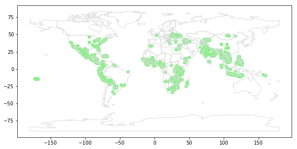
- 세계 지도를 일단 가져오자.
- 이정보는 GeoPandas가 제공한다.
# This dataset is provided in GeoPandas
world_filepath = gpd.datasets.get_path('naturalearth_lowres')
world = gpd.read_file(world_filepath)
world.head()
- 세계 지도에 loan이 있는 위치만 표시해보자
# Your code here
ax = world.plot(figsize=(10,10), color='none', edgecolor='gainsboro', zorder=3)
world_loans.plot(color='lightgreen', ax=ax)
- 그러면 다음과 같은 지도가 생성되게 된다.
3) Select loans based in the Philippines.
- 일단 그럼 필리핀에 있는 loan 정보들만 따로 모아보자.
# Your code here
PHL_loans = world_loans.loc[world_loans.country.isin(['Philippines'])].copy()
4) Understand loans in the Philippines.
- 필리핀 지도를 받아오고
# Load a KML file containing island boundaries
gpd.io.file.fiona.drvsupport.supported_drivers['KML'] = 'rw'
PHL = gpd.read_file("../input/geospatial-learn-course-data/Philippines_AL258.kml", driver='KML')
PHL.head()
- 여기에 필리핀 loans를 띄워보자.
# Your code here
ax = PHL.plot(figsize=(10,10), color='none', edgecolor='gainsboro', zorder=3)
PHL_loans.plot(color='gray', ax=ax)
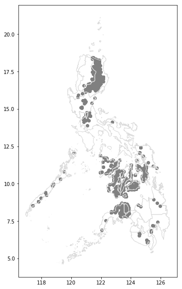

- 우리가 만든 맵과 실제 지도를 대조해본다면 Mindoro라는 지역이 넓은데 후원의 흔적이 없으므로 여기를 추천하도록 하자!
- 이상으로 첫 Tutorial을 마치겠다.
이 포스팅은 쿠팡 파트너스 활동의 일환으로, 이에 따른 일정액의 수수료를 제공받습니다.
Subscribe via RSS